Getting Started in Data Science: R vs Python

Image – Wikimedia Commons

Introduction

Every person that starts out working with data in any serious capacity eventually asks “what language should I learn for data science?” Often the choice is difficult to make and there is a lot of strong opinions out there regarding what tools are needed for data science. In this post, we will discuss why you cannot just use Excel (the need for programming), discuss Python and R and how you should choose which to learn.

Why Can’t I Just Use Excel?

As mentioned in the introduction, doing anything serious with data requires more than just Microsoft Excel. There are a lot of “data analysts” who just simply use Excel. Normally, these analysts are not really doing anything statistically meaningful. They may be making some graphs, calculating some summary statistics or even visually looking at the data for patterns. There are probably others as well that do some interesting things with Excel (we often embed ML models in Excel workbooks), however Excel is not a very deep tool as far as analysis goes.

With Excel, you lack reproducibility, flexibility and lack more advanced concepts. Reproducibility refers to being able to reproduce an analysis for confirmation of results. This means that no one can recreate results you achieved with your workbook. This may be possible with VBA, but not for most people that do not know VBA. In some business settings, this may be OK, but is a huge red flag in academic or trade settings where peer review matters.

When it comes to flexibility, you are stuck with what Excel has to offer in the form of functions and structure. Writing your own functions in Excel is possible, but most people do not know how to do it. There is quite a bit of flexibility in Excel’s VBA, but this is another programming language that most people do not know how to use and it is not exactly straightforward. Excel can also make data visualizations, but handcrafting the graph to get it the way you want is easier said than done with Excel. Then that process has to be repeated for multiple graphs. Excel also slows down if it works at all with really large amounts of data.

Last, Excel has many data analysis functions built in for hypothesis tests, ANOVA, Fourier analysis etc… but is lacking many advanced data science techniques such as machine learning concepts. When it comes down to it, Excel is not meant for really sophisticated data analysis. It is meant as a spreadsheet tool for getting quick insights or answers out of data, not deep insights via pattern recognition. This means that we need a way to analyze data with sophisticated methods in a reproducible and flexible way, this means we need to program.

This is often the hardest pill for people to swallow that are analysts, but may not consider themselves programmers. Programming is a skill that can be learned by anyone. It is simple passing the computer instructions similar to how you would with a mouse or a keyboard. It does take time to master, but increases the scope of what is possible. In data science, the two most important programming languages are R and Python.

Python

Python was invented in 1991 by Guido Van Rossum and is named after the British Comedy group Monty Python. It is an object oriented programming language that is used in data science, but is also a general purpose language used in gaming, web development and application development. You can do almost anything with Python (RealPython). It is used heavily in data science by a lot of companies and most people that end up using Python for data science come from the computer science school of thought. Python is an easy language to learn and can be rather efficient. It uses multiple CPU’s natively and is therefore fast. As far as data science goes, there are multiple packages to support data science type work. Pandas is used for data manipulation and structuring, scikit-learn is used for machine learning, Keras and Tensorflow are used for deep learning, statsmodels is used for statistical modelling and packages such as seaborn and Dash are used for data visualization and dashboards. Data scientists often use IDE’s such as Spyder, Rodeo and PyCharm.  Python is also open source, so cost is not an issue here.

Python does have its disadvantages. Some of the packages developed are not as mathematically rigorous as packages developed in R since many are developed my programmers, not statisticians. There is some risk with that. Also, applying packages can often be frustrating in trying to find and assess functionality. Almost everything done with Python is through a package add on. With some data science related work, simple functionality often becomes a lot more difficult. For example creating a plot with matplotlib is numerous lines of code to get the plot in a place that is acceptable. Understanding the nuances between lists, dictionaries, tuples and dataframes also gets quite a bit frustrating in reshaping of data. Python at times can also have weak or non-existent documentation. R has standards around package documentation that are much more stringent.

R

R was developed as a successor to S developed by John Chambers at Bell Laboratories for statistical processing (Rproject). R was specifically built for statisticians by statisticians. This is both its strength and weakness. R is often popular in academic settings and settings closely bound to academia. Unlike Python, R offers a lot of strong functionality in its base packages such as statistical modelling, linear modelling, plotting, statistical computations and hypothesis testing and even some classification out of the box. Outside of that, R packages are strongly vetted before being placed on the CRAN environment to download. Packages such as Caret are general purpose machine learning packages, NNET and H2O are deep learning packages, ggplot is the golden standard of plotting, dplyr and data.table are amazing data manipulation packages and Shiny and Plotly are used for interactive apps and plots. RStudio is the IDE for R and is one of the best IDE’s to work in for data analysis. R is also open source and free like Python which means anyone can extend and add to it.  

R, like Python has its disadvantages. Since it was written by statisticians, programmers often find R’s syntax and paradigms difficult to learn and understand. However, many people that are not programmers often find it more intuitive. R only runs on single CPU’s out of the box which makes it slower than Python. There are some packages that allow a user to utilize more CPU’s and some do it out of the box such as data.table. R is often more difficult, but not impossible, to implement in an application or website flow. Python is much more easily integrated into architecture.

Should I Choose R or Python?

The answer to this is that it depends. In most people’s cases, I would recommend both. R has strong statistical theory and ease of implementing concepts behind it, while Python has the advantage of speed and integration capability into most software stacks. Often, I choose to do data analysis in R and then build general purpose programs for things like web scraping in Python. Deep Learning is also better in Python due to its speed out of the box. If you do not want to learn both, then the recommendation would be to learn R if academia or research is the goal and learn Python if a job in a business setting is the goal. Either way, the methods and skills gained by learning either cannot be replaced.

In conclusion, both languages have their pros and cons and both are very good languages. It depends on the arc in which you envision your career to progress that would drive your decision. Both languages are open source and free and have a lot of resources behind them to help someone get started and support the users. Remember we offer training in both R and Python. This can be requested at Courses .

Machine Learning 101: All the Basics You Need to Know

Introduction

In this blog post, we will discuss machine learning. We will answer a simple question, what is machine learning? Then we will describe the elements of machine learning along with some common terminology to understand. After that, we can discuss the machine learning process. Last, we will discuss some machine learning applications. This is truly an exciting field that everyone in business should have this elementary understanding of. Let’s get started!

What is Machine Learning?

Simply put, machine learning is a field in artificial intelligence. Some may be surprised to hear this, but artificial intelligence is not just one thing, rather it is a general term for a combination of different approaches and tools that is meant to mimic human intelligence. Machine learning can be thought of as the field that represents how humans learn from experience. Arguably, machine learning can be thought of as part of the brain in artificial intelligence. 

The way humans learn is from acquiring knowledge from their environment or being told knowledge from other people. The brain retains this knowledge and uses it in future decision making and interaction with the world. Machine learning works the same way. Machine learning takes data (experience) and relates it to an outcome. Then it learns from this data and is able to make predictions (decisions) on new data that is presented. This is different than programming as no instructions are ever provided to the model for its decision-making process. Rather it is learning the underlying pattern within the data and storing this model for future use. Think of it as reading a book then taking a test on the topics within the book. You are extrapolating what you learned in a book to answer unseen questions about the book.

The theoretical idea behind machine learning is that there is a single best mathematical function that best represents the pattern within the data. The goal of the data scientist is to try to figure out what this underlying theoretical function is by searching a large space of existing functions. The formula of linear regression from our blog post is an example of such a function De-mystifying Simple Linear Regression. This must be done because you will never know the underlying function of the problem that is being solved, but it can be approximated. There is a lot more theory behind machine learning, but that is for another post.

To sum up, machine learning is the process teaching a computer to learn a pattern from a given dataset and using that experience to make predictions (decisions) when given new data. 

Elements of Machine Learning

Machine learning is often referred to by different terms that are very similar, if not the exact same as machine learning. Predictive analytics, data mining, statistical learning and deep learning are just synonymous terms or types of machine learning. Now, let’s break down machine learning into a few pieces. 

There are two types of machine learning, supervised and unsupervised learning. 

Supervised Learning

First, supervised learning means we have a data set with input data and we know the output that we are trying to model. The output or dependent variable is typically referred to as Y. Now, we only know the output for our observed data set. If we knew all Y outputs, then we would not need machine learning. However, the model will learn what patterns in the data create the Y output and build the function to approximate this pattern. Then unseen data can be passed in and predicted. 

With supervised learning, we are trying to do one of two things. Either predict a continuous output (a number) or predict a class (non-numeric data). This is known as regression and classification. These terms refer to the type of the problem we are trying to solve based on the type of the output or Y. 

Regression

This term is often confusing as this encompasses models that are different than linear regression, which we are all familiar with. Basically, regression means we are trying to predict a number as the output or Y variable. This could be a price, temperature, weight or anything that has a numerical scale. While linear regression is not the only model when regression is our problem type, many regression models use linear regression or rather the assumption of linearity as their base. Again, this is outside the scope of this post. Ultimate takeaway is when trying to predict a number, a regression-based model is used. 

Classification

This is often referred to as pattern recognition. This means that we have at least two classes (often more) as our output and we are trying to find the pattern to probabilistically assign the label (Y) to the data. When we say class or label, think of groups or types of things. For example, a type of snake (poisonous or not-poisonous), the outcome of a marketing campaign (purchased our product or did not purchase our product), groups of temperatures (frozen, cold, neutral, hot, boiling). These categories can often be arbitrarily assigned or even represent human emotion or feeling. When classification is the problem type, the type of model used will be different as well as the output. Ultimate takeaway is when trying to predict groups or classes of data including words, a classification based model is used. 
To recap, supervised learning means we use the outcome or Y variable to train the model. We can have either a regression or classification type of problem to solve and each of those two problem types have different types of models that can be used. 

Unsupervised Learning

This is the opposite of supervised learning as in this case, we do not have a Y variable or output to use for training the model. This means that a whole different set of models must be used on the dataset. Often unsupervised learning is used as a way to generate classes or labels for a dataset that is then used for supervised learning. Since the output here is not known, the model finds the best way to group the data and build the labels. If not being used for supervised learning, this can be used to understand what types of categories exist in a dataset. This is often used in computer vision as well to build versions of simpler images by grouping colors. Ultimate takeaway is unsupervised learning is used to let the computer determine the best way to group observations in a dataset. 

Semi-Supervised Learning

Semi-supervised learning falls somewhere between supervised and unsupervised learning. This means you will have labels for some observations but not for all. Often what happens is it can be difficult or costly to build an entire training set for a supervised learning algorithm, so people will classify a small section of the data and use supervised learning to label the rest of the data before training. Often, only the most confident observations are kept and the uncertain examples discarded. This provides a larger training set that is not hand classified. It should be noted that this does build uncertainty into the model more so than hand labeling a dataset will. 

The Machine Learning Process

The machine learning process can be visualized as follows:

First, the problem is defined. What are we trying to accomplish with machine learning? For example, can we predict which customers will churn from our subscription service based on prior behavior? The problem must be specific enough to gather data and solve. Then we gather training data. What variables are important or could be and what data exists? From there, do we know the output or not? If we do not know the output do we want to hand classify the data or use unsupervised learning? If we use unsupervised learning, then we run a variety of unsupervised models and review. We then decide if we want to use these to train a supervised model or we are done! For supervised models, we select models to train based on our problem and try to find the model that best approximates our output. We test to see which model achieves the best tradeoff between bias and variance (complexity vs non-complexity).  The best model will be the one that generalizes the best on unseen data, not the one that trains the best. Once, we have our model, we predict on new data! This is an oversimplification of the process, but it provides a high-level overview of what happens in the machine learning process. This is key to understand. 

What Can You do With Machine Learning?

There are so many applications in machine learning that they cannot all be listed. Here are a couple:

Marketing Applications

Machine learning fits nicely into the marketing research process and provides additional sophistication and accuracy to a marketing research problem. This could include applications such as predicting customer churn, lifetime revenue of a customer and predictive, targeted marketing. Individuality of consumers can be maintained and marketed using machine learning. Recommendation systems are a popular example of machine learning in marketing. Think about recommendations Netflix provides based on your prior watching history. 

Finance Fraud / IT Security

 Banks and the finance industry use a lot of machine learning to catch fraudulent transactions on a banking or credit card account. This is why sometimes your credit card is frozen and you get a call from your bank to validate charges. Information technology is in a similar situation. It uses machine learning to identify a hacker’s presence in their network or again to identify fraudulent transactions. Banks also use machine learning to vet loan applications based on customer demographics. This can often be controversial. 

Supply Chain / Manufacturing Applications

There is a lot of data that flows through a supply chain and manufacturing plants. In the supply chain, dates of arrival of freight can be predicted using weather patterns, carrier patterns and port capacity. Forecasting can also be enhanced using more advanced predictive models. In the manufacturing plant, quality defects can be predicted based on machine performance data. Also, machine breakdowns can be predicted so the machines can be scheduled for maintenance when they need it and avoid downtime. 

Process Automation

This is a generic catch-all, but basically any process that is repetitive or contains human decision points can be automated with machine learning. Machine learning is consuming a lot of manual work in marketing, accounting and project management functions. This is because machine learning can replicate a human and actually make more consistent decisions than a human can.

Conclusion

Machine learning is an extremely powerful tool and is transforming the way business is done. Usually when people refer to artificial intelligence, they usually mean machine learning. There is a lot of advanced math that goes into machine learning and takes time to understand. However, it is important everyone understands machine learning especially as it grows in popularity. This is so change can be embraced and the technology is not feared, but embraced and used to create more accurate and efficient operations. We will be expanding our posts on machine learning and concepts related to machine learning as we continue on our mission to change the ways companies operate and become data-driven. Stay tuned!
 

What You Need to Know About AI’s Impact on the Workforce

A common belief that we have encountered in our field is that artificial intelligence is “the enemy”. This has been the result of a fear that embracing this technology will lead to an unemployed human race.

This is nothing new and this fear has applied to various emerging technologies throughout history. Many AI proponents have referenced the book “Learning by Doing: The Real Connection between Innovation, Wages, and Wealth” when defending AI. In the “non-missing bank tellers” section of the book, James Bessen discusses the initial objection to the implementation of ATM machines during the 1970s. Critics reasoned that since ATMs would be responsible for handling transactions, then bank tellers would become obsolete, but statistics from the Bureau of Labor, showed this was not the case.  The ATMs did result in the need for less bank tellers at each branch office. However, because it became cheaper to operate branch offices, the cost reduction allowed for branch expansion and more jobs were created in the process.

AI detractors would argue that there are instances where technology has been known to destroy jobs. For example, Venturebeat.com reported that a Deloitte study of automation in the U.K. found that 800,000 low skill level jobs were eliminated as the result of AI and other automation technologies, but as Professor Robert Gordon of Northwestern University, has stated “though jobs are constantly being destroyed, they are also being created in even larger numbers”. In the UK case, 3.5 million new jobs were created and those jobs paid on average nearly $13,000 more per year than the jobs that were lost. Gordon also stated, “No invention in the last 250 years, since the first Industrial Revolution, has caused mass unemployment.  – there is enormous churn in the job market – at present, there is actually a shortage of workers, not a shortage of jobs, even in fields such as construction, skilled manufacturing and long-distance truck driving”

Nevertheless, as we stated in a previous blog, AI should not be used as a reason to fire people. Instead, companies must adopt strategies such as: simultaneous operating designs and repurposing instead of waiting to see what the impact will or will not be on their workforce. It is imperative that companies invest in their employees so that they can adapt to the unyielding AI revolution. Employees must seek and not decline to improve their skillsets. The businesses that manage new technology properly will have the highest productivity from technology and the workforce.

Ultimately, we should not reject innovation due to fears. When one door closes another one opens…the question is, will you be ready to walk through?

References

1. Bessen, J. (2015). Learning by doing: the real connection between innovation, wages, and wealth. New Haven: Yale University Press.

2. Ghafourifar, E. A. (2017, September 07). Automation replaced 800,000 workers... then created 3.5 million new jobs. Retrieved March 09, 2018, from https://venturebeat.com/2017/09/07/automation-replaced-800000-workers-then-created-3-5-million-new-jobs/

3. Kochan, T. A., & Dyer, L. (2017). Shaping the future of work: a handbook for action and a new social contract. Boston: MITx Press.

4. Productivity Know How. (2018, January 24).  AI to create millions of jobs. Retrieved March 01, 2018, from http://productivityknowhow.com/ai-increase-process-productivity/

De-mystifying Linear Regression Part 2

Introduction

In our last post, we introduced simple linear regression and how to calculate simple linear regression using the least squares method. This was from a pure mathematical perspective. In this post, we will discuss using the linear regression model from the last post and using it to make predictions. Then some pro's and con's of linear regression will be discussed. The assumptions of a linear model, diagnosing fit of a model and computing computationally will be left to another blog post.

Recap

From the first post in this blog series, we took a theoretical heating and cooling repair company and took their hours spent on the job data and used it to model the cost based on the amount of hours needed for a job. We expect our client to plug in a job hours estimate and be able to get out an estimated cost. This cost could vary based on labor and parts, which is a discussion for a different time, but for the purpose of this conversation, we are just going to use job hours.

As a reminder, here is a plot of the data:

We then fit a simple linear regression model using least squares. When we do that, we come up with the equation:

When we plot this line to the data, we get:

The steps to do this are discussed in the last post, but we can see that the line appears to fit the data pretty well. Our model statistics would confirm this, which is a different post on evaluating models.

Making Predictions

Usually in simple linear regression, the model would be evaluated before predictions are made, however this writing is just meant to provide an overview of simple linear regression and to show the predictive nature of linear regression models.

Now the company has their model built, so the first thing they want to do is take it for a test spin and estimate some job costs.

Using the linear regression function, making a prediction is as simple as plugging in x. Recall our equation is:

So if we wanted to predict cost for a 4.5 hour job, we would plug in 4.5 for x:

Which gives:

453.87 rounding to two decimal places.

Since our cost for a 4 hour job is around $400 and the cost for a 5 hour job is $500, this seems very logical.

Plotting this estimate on the graph in red gives:

Using our gut judgement, that value seems very likely. Its probably pretty unlikely that this exact value will be the actual cost and many people would use a prediction interval to show the range of possible predictions for this value. However, in real life, an actual number to estimate a response is required. The prediction value usually falls in the center of that prediction interval to give a generalized value, almost like finding the average of a range of possible prediction values.

What about values that are outside of the range of data we have? What if the business wants to know how much a 9 hour job or a 12 hour job would take? We can run this through our model as the x variable in the same fashion. This gives:

The estimated cost for a 9 hour job is 895.1141

The estimated cost for a 12 hour job is 1189.279

These estimates sound likely according to our model, but there is a theoretical question here. Do we really expect the same data trend to continue with jobs that long? For example, both jobs exceed 8 hours, so wouldn't there be additional costs for a job spanning into 2 days? These questions are really unanswerable without data, but industry experience can be used to supplement the lack of data. If the experts of this situation think the model would remain consistent, then this extrapolation would be fine. There are many statisticians that would argue against extrapolating a model, but if the extrapolation is certain, there is nothing wrong here. However, if the company is unsure if the pattern would hold, the data should not be extrapolated and the model should only be used as a guideline, if at all.

Breaking Down the Equations and Results

Recall that our equation to fit this model is:

In this situation we can translate our coefficients into actual values that mean something. First, since Beta_0 represents a cost when our work is zero, we can think of this as the fixed cost portion of the model. This means a job costs $12.6 regardless of the work done. This would cover pieces of the business not dependent on the job such as the company owned building.

Next, the Beta_1 coefficient, which is 98.0551331, represents the rate of change which is completely variable. This number means a typical service job costs around $99 an hour including parts and labor. This number depends on the length of the job, which is the variable piece.

It is easy to see why this information is useful to our business. While this is a simplified example of how a business can make use of a linear model, it is an effective method and model. The business does not need to know the exact cost of parts and labor, just provide an hour estimation.

Pros and Cons of Simple Linear Regression

There are a lot of reasons why linear regression is a good model to use in predictive analytics and machine learning.

1.          The model is interpretable - With the simple example, the model and the coefficients make sense. They are easy to understand and can be used to predict and are easy to explain. This makes linear regression one of the best models to use even though more accurate options may exist.

2.          The model has low variance - This means that as data points are replaced and the training data changed, the model will only shift slightly. This gives a consistent result model to model with a small amount of change between each model. Low variance is a desired quality in machine learning.

3.          Linear regression can be expanded to use multiple parameters - Multiple linear regression takes multiple input parameters and can produce an even more accurate estimate. In our example, there are probably other input parameters that affect the cost of a job, so once captured they can be used to predict a more accurate cost. Note that some relationships are quadratic or cubic, these can also be fit using linear regression.

While there are some pros to linear regression, it also has its shortcomings:

1.          It is inflexible - Linear regression fits a straight line to a dataset. Very few real world examples are purely linear. There are usually more complicated relationships between variables. There are often curves and shifts in data that cannot be modeled with a simple linear regression function.

2.          It exhibits high bias - Bias is a statistical property that indicates how much error is introduced by trying to model a complex situation with a simple model. It is the average of the difference between actual values and the predicted values, this should come out as 0 in a perfect model. The model may exhibit low variance, but will produce high bias since it cannot accommodate patterns in the data that may emerge. Ideally, both variance and bias should be minimized. This results from the inflexibility of the model.

Conclusion

Simple linear regression is a great tool. It is often used in other machine learning models and neural networks. The machine learning community has downplayed it's importance, but if the model fits and predicts well, then use it. A simple model that can be explained is often more valuable than a complex model that cannot be explained. For more complicated models, multiple linear regression can be valuable as well. What we did not cover in this writing was how to determine if the model is adequate. We will discuss this in a different post on linear regression model adequacy. We will also discuss multiple linear regression in a future post.

De-mystifying Linear Regression Part 1

Introduction

In our last post, we discussed the scientific method and how it has been adopted for business use cases. While there are numerous variations of the scientific method in business, most philosophies take a similar approach to solving business problems and driving exploration. In this post, we will continue our discussion of data science and statistics tools and techniques and discuss linear regression as it applies to machine learning.

Definition

Before diving in, let's get some terminology out of the way. In the wild, it is possible that multiple terms could be used simultaneously for related, but different things. For example, in machine learning there are two major types of supervised learning problems, a regression problem and a classification problem. Regression refers to predicting a numerical value while classification refers to predicting a descriptor of the data or a classifier. Linear regression is a form of a regression model in machine learning, but there are other types of algorithms that can be used for regression learning such as Random Forest and Support Vector Machines. This writing will focus on the Simple Linear Regression algorithm and leave regression problem types to discuss at a later date.

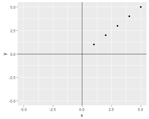
Simple Linear Regression is really a mathematical formula that is meant to determine the relationship between two variable, an X or predictor and a Y or an outcome. Simple linear regression is called simple because it only has one predictor. Remember back to algebra in high school where as a student you were required to find the slope of a line in a cartesian plane. An example of a cartesian plane and some points are shown below.

Remember in a cartesian plane, x represents the horizontal axis and Y represents the vertical axis. In the plot shown, there are a series on points in the 1st quadrant. Back in algebra, often the problem would instruct a student to find the slope of this series of points or even a line. Remember, the formula for slope is given as:

With mx representing the slope and b representing the Y intercept (the Y point when X is 0). Remember, slope is simply:

Rise being how much the line changes on the y axis from point to point and run being how much the line changes on the x axis from point to point. So if we take the first two points (1,1) and (2,2), we see that the slope is:

Fitting a line to this data is simple because the slope is the same point to point so the regression line looks like:

Then if we say that the slope of the line is 1, what is the value of Y when X is 6?

If you said 6, then just did your first machine learning prediction. We have no reason to believe that Y would not be 6 if X was 6 based on the sample of data we have here. This was an overly simplistic example, lets look at another more complicated example.

Let's say we have a theoretical company whose service is heating and cooling repair. They perform house calls and can spend various amounts of time at a job depending on the complexity. Well they have collected some data from their past 19 service calls and would like to see if they can build a model to help them better quote jobs when customer's ask for costs. There could be a large amount of variables here for them to do that, but they noticed there seems to be a relationship between how long a job takes and how much it costs the customer. Since the actual cost is unknown until the technician diagnoses the problem, most of the time the customer service rep can estimate how much time a job will take based on the symptoms of the problem. Below is a table of the collected data:

##    Job_Length_hours Cost_in_$$
## 1               1.0        100
## 2               3.0        280
## 3               6.0        610
## 4               0.5         50
## 5               0.5         80
## 6               2.0        200
## 7               2.0        200
## 8               3.0        302
## 9               5.0        498
## 10              1.0        111
## 11              1.5        145
## 12              1.0        100
## 13              2.0        198
## 14              3.0        320
## 15              4.0        406
## 16              2.0        250
## 17              1.0        160
## 18              1.0         80
## 19              1.5        170

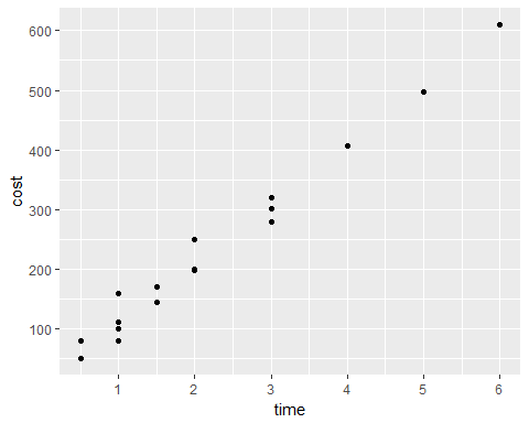
It is important to note that the cost is the response and the job length is the predictor. First thing we should do is plot these points (only showing the first quadrant of the Cartesian plane):

What is quickly noticed is that as time increases, so does the cost. However, we cannot just simply take the slope here because at some points there are different costs tied to the same amount of time. For example, if a job takes 3 hours, the costs have ranged from $280 to $320. So how would we go about modeling this?

First, let's define the simple linear regression equation as:

Y - The response value in the dataset.

β_0 - The value of Y when X is zero, the Y-intercept.

β_1 - The estimated slope coefficient.

X_i - the value of X at observation i.

ϵ_i - the error of the fitted regression model at observation i. In other words, error that is unexplained after a model is fit.

i=1,2....k - i is the number of observations in the dataset running in this case from 1 to 19.

Do not let the Greek letters intimidate you. These are just placeholders for coefficients that will be estimated.

Fitting the Simple Linear Regression Model

Now we will use something called least squares linear regression to calculate the model. Least squares is the most commonly used form of linear regression. It works by minimizing the sum of the squared deviations between the actual data and the model to estimate the coefficients. To fit a least squares linear regression model, the following steps will be performed:

1.          Calculate the mean of the x's or predictor variable.

2.          Calculate the mean of the y's or outcome variable.

3.          Calculate the standard deviation of the x's or predictor variable.

4.          Calculate the standard deviation of the y's or outcome variable.

5.          Calculate the correlation coefficient of x and y.

6.          Calculate the slope coefficient.

7.          Calculate the y-intercept or  coefficient.

8.          Put it all together in a nice formula.

If you are reading those steps and do not know how to do any of them, that's ok, we will do them now!

Calculating the Mean (Statistical Average) of X and Y.

The mean is just the statistical average of a data set. Most people have experience calculating the mean and use it as an estimator for everything, which leads to a lot of unexpected events. First, to calculate the mean of x, we will use the formula:

This just means, we are going to add up all of the x's and divide by the number of observations. So adding up all of the values in Job_Length_hours column we get:

1+3+6+0.5+0.5+2+2+3+5+1+1.5+1+2+3+4+2+1+1+1.5 = 41

Next, we have 20 observations, so we divide the sum of x by the number of observations to get:

Notice, we do not want to round yet if we can help it. Also notice that the mean of x is denoted as ¯x.If the process is repeated for y, we have 224.2105. See if you can replicate the calculation to get y on your own. If you are using excel, you can just use the average function. I typically use R which uses the mean() function.

Calculating the Standard Deviation of X and Y.

The standard deviation is a little more complicated. Also notice we found the mean of x and y first; that is because we will need it as an input into the standard deviation. The standard deviation is found by:

What we are doing here is first calculating the variance under the square root and then taking the square root of that number to find the standard deviation. Note the standard deviation is a calculation thatr essentially finds the average distance of points from the mean or average. This is done by subtracting the mean of x from each actual observation, squaring it and then adding up all of those points. Then divide the sum of squares by n and take the square root. Let's do x together.

First, subtract the mean from each x point. Remember the mean is 2.157895. It might make sense to do this in a table to avoid confusion:

##    time    meanx       Diff
## 1   1.0 2.157895 -1.1578947
## 2   3.0 2.157895  0.8421053
## 3   6.0 2.157895  3.8421053
## 4   0.5 2.157895 -1.6578947
## 5   0.5 2.157895 -1.6578947
## 6   2.0 2.157895 -0.1578947
## 7   2.0 2.157895 -0.1578947
## 8   3.0 2.157895  0.8421053
## 9   5.0 2.157895  2.8421053
## 10  1.0 2.157895 -1.1578947
## 11  1.5 2.157895 -0.6578947
## 12  1.0 2.157895 -1.1578947
## 13  2.0 2.157895 -0.1578947
## 14  3.0 2.157895  0.8421053
## 15  4.0 2.157895  1.8421053
## 16  2.0 2.157895 -0.1578947
## 17  1.0 2.157895 -1.1578947
## 18  1.0 2.157895 -1.1578947
## 19  1.5 2.157895 -0.6578947

Taking the first value and performing the calculation 1-2.157895 = -1.1578947.This operation is repeated for each value of job time. Next step is to take the values we calculated in the new column and square them.

##    time    meanx       Diff     Squares
## 1   1.0 2.157895 -1.1578947  1.34072022
## 2   3.0 2.157895  0.8421053  0.70914127
## 3   6.0 2.157895  3.8421053 14.76177285
## 4   0.5 2.157895 -1.6578947  2.74861496
## 5   0.5 2.157895 -1.6578947  2.74861496
## 6   2.0 2.157895 -0.1578947  0.02493075
## 7   2.0 2.157895 -0.1578947  0.02493075
## 8   3.0 2.157895  0.8421053  0.70914127
## 9   5.0 2.157895  2.8421053  8.07756233
## 10  1.0 2.157895 -1.1578947  1.34072022
## 11  1.5 2.157895 -0.6578947  0.43282548
## 12  1.0 2.157895 -1.1578947  1.34072022
## 13  2.0 2.157895 -0.1578947  0.02493075
## 14  3.0 2.157895  0.8421053  0.70914127
## 15  4.0 2.157895  1.8421053  3.39335180
## 16  2.0 2.157895 -0.1578947  0.02493075
## 17  1.0 2.157895 -1.1578947  1.34072022
## 18  1.0 2.157895 -1.1578947  1.34072022
## 19  1.5 2.157895 -0.6578947  0.43282548

For example, take the first calculated value and multiply it by itself: -1.1578947*-1.1578947 = 1.34072022. Repeat this for all values calculated in the Diff column.

Next, sum up all values in the squares column, divide by n-1 (18) and take the square root:

## [1] 1.518887

Summing the squares column gives 41.52632 (feel free to check). Then dividing 41.52632 by 18 gives:

Last taking the square root of this gives:

That's it! Standard deviation has been calculated. Repeating for y gives 150.3066.

Calculating the Correlation Coefficient of X and Y

The correlation coefficient is meant to measure the linear relationship by x and y. The value falls between -1 and 1. If the value is at or around 0, there is no linear relationship. If the value is closer to 1 or -1, then there is a strong positive or negative relationship or slope. Calculating this coefficient uses the mean and standard deviation from the previous exercises.

The first step is the same as in calculating standard deviation, the mean is subtracted from each value of x and y, so we will skip that since it was done for standard deviation. Since we have that value, next we are going to divide by the standard deviation to get a standardized value.

##    time    meanx       Diff     Squares Stand_Dev Standard_Value
## 1   1.0 2.157895 -1.1578947  1.34072022  1.518887     -0.7623311
## 2   3.0 2.157895  0.8421053  0.70914127  1.518887      0.5544226
## 3   6.0 2.157895  3.8421053 14.76177285  1.518887      2.5295532
## 4   0.5 2.157895 -1.6578947  2.74861496  1.518887     -1.0915195
## 5   0.5 2.157895 -1.6578947  2.74861496  1.518887     -1.0915195
## 6   2.0 2.157895 -0.1578947  0.02493075  1.518887     -0.1039542
## 7   2.0 2.157895 -0.1578947  0.02493075  1.518887     -0.1039542
## 8   3.0 2.157895  0.8421053  0.70914127  1.518887      0.5544226
## 9   5.0 2.157895  2.8421053  8.07756233  1.518887      1.8711763
## 10  1.0 2.157895 -1.1578947  1.34072022  1.518887     -0.7623311
## 11  1.5 2.157895 -0.6578947  0.43282548  1.518887     -0.4331427
## 12  1.0 2.157895 -1.1578947  1.34072022  1.518887     -0.7623311
## 13  2.0 2.157895 -0.1578947  0.02493075  1.518887     -0.1039542
## 14  3.0 2.157895  0.8421053  0.70914127  1.518887      0.5544226
## 15  4.0 2.157895  1.8421053  3.39335180  1.518887      1.2127995
## 16  2.0 2.157895 -0.1578947  0.02493075  1.518887     -0.1039542
## 17  1.0 2.157895 -1.1578947  1.34072022  1.518887     -0.7623311
## 18  1.0 2.157895 -1.1578947  1.34072022  1.518887     -0.7623311
## 19  1.5 2.157895 -0.6578947  0.43282548  1.518887     -0.4331427

Walking through the first x value, subtract the mean from x, then divide the difference by the standard deviation to get the standard value.

Repeat this for every value of x. Before moving on, it is important to calculate the y values as well.

##    Standard_Value_X Standard_Value_Y
## 1        -0.7623311       -0.8263812
## 2         0.5544226        0.3711712
## 3         2.5295532        2.5666841
## 4        -1.0915195       -1.1590347
## 5        -1.0915195       -0.9594426
## 6        -0.1039542       -0.1610743
## 7        -0.1039542       -0.1610743
## 8         0.5544226        0.5175388
## 9         1.8711763        1.8215403
## 10       -0.7623311       -0.7531975
## 11       -0.4331427       -0.5269931
## 12       -0.7623311       -0.8263812
## 13       -0.1039542       -0.1743804
## 14        0.5544226        0.6372940
## 15        1.2127995        1.2094580
## 16       -0.1039542        0.1715792
## 17       -0.7623311       -0.4271971
## 18       -0.7623311       -0.9594426
## 19       -0.4331427       -0.3606664

Now we have the standard values of x and y in a table. Next, we multiply the standard values of each x and each y.

##    Standard_Value_X Standard_Value_Y     Product
## 1        -0.7623311       -0.8263812  0.62997610
## 2         0.5544226        0.3711712  0.20578572
## 3         2.5295532        2.5666841  6.49256380
## 4        -1.0915195       -1.1590347  1.26510898
## 5        -1.0915195       -0.9594426  1.04725034
## 6        -0.1039542       -0.1610743  0.01674436
## 7        -0.1039542       -0.1610743  0.01674436
## 8         0.5544226        0.5175388  0.28693519
## 9         1.8711763        1.8215403  3.40842309
## 10       -0.7623311       -0.7531975  0.57418585
## 11       -0.4331427       -0.5269931  0.22826320
## 12       -0.7623311       -0.8263812  0.62997610
## 13       -0.1039542       -0.1743804  0.01812759
## 14        0.5544226        0.6372940  0.35333020
## 15        1.2127995        1.2094580  1.46682995
## 16       -0.1039542        0.1715792 -0.01783638
## 17       -0.7623311       -0.4271971  0.32566561
## 18       -0.7623311       -0.9594426  0.73141293
## 19       -0.4331427       -0.3606664  0.15622000

Taking the first entry, multiply -0.7623311*-0.8263812 = 0.62997610. Repeat for each value of X. The last step is to sum up the new column of products and divide by n-1. Summing the products gives 17.83571. Dividing that by 18 yields a correlation coefficient of 0.9908726.This tells us our data set has a really strong positive correlation.

Calculate the Slope Coefficient

Whewwwww...Almost there. The slope coefficient or β_1 is found by multiplying the correlation coefficient by the ratio of standard deviations of y and x or:

That was not too bad, let's move on to find the y intercept or β_0.

Calculate the Y intercept

The y intercept or β_0 is found by:

So that is the mean of y minus the product of the slope coefficient and mean of x:

224.2105263 - 98.0551331 * 2.1578947 = 12.6178707

Assemble the Linear Equation

To assemble the linear equation, plug in the values for β_0 and β_1. Which is:

This is the formula that can now be used to predict other values. Plugging in all of the current values for X will give the fitted values of the model so we can evaluate model fit.
For example, the first value of x is 1, so we have:

Y_1=12.61787+98.05513*1=110.67300

Repeating this for all values of x, provides the fitted values of the model. Now let's plot our model against our data to see the fit:

Conclusion

Since this post is already running long, we will leave it there. In our next post, we will continue this concept and assess the fit of the model and start predicting some future values. We will also discuss the pro's and con's of simple linear regression.

4 Ways the Scientific Method is Used in Business

In this post, we will discuss the scientific method and how it is applied in business, process science and data science. This key fundamental drives a lot of the thinking about improvement, optimization, formalizing problems and using evidence and data to make decisions.

What is the Scientific Method?

Think back to elementary school. Every year most schools have something called the “Science Fair”. You would have to get one of those big tri-fold display boards and decorate it with some type of experiment you were supposed to carry out. Basically, this is a way for children to come up with a problem or theory to test, test the theory and then present the data as conclusions. The whole point of this is to instill the scientific method into children.  The principles of this exercise are used by adults in research and industry, although they have traded out the tri-fold displays for PowerPoints and white papers.  Let’s explore the scientific method in a little more detail.

There are many variants and wordings for the scientific method. For the purpose of this writing, we will stick to five major steps.

1.       Identify the problem or question – This step is the beginning of the entire process. What are you trying to solve? These questions or problems usually come from observed phenomena. Over the years people have asked questions such as what are clouds made of? How do birds fly? Why did the apple fall from the tree and hit me in the head? That last question specifically led to the discovery of gravity, all from asking a question. A clear, well formulated problem or question needs to be specific enough to be tested and proven or disproven.  

2.       Hypothesis – Now that there is a question or problem to solve, this step seeks to address the question and formulate a theory to test. Basically, the experimenter must come up with a potential reason for the observed phenomena. This is usually something driven by the evidence on hand so far. Getting the hypothesis usually requires some thinking, knowledge or possibly existing data. This theory must be explicitly stated and able to be tested. If it cannot be tested, it cannot be proven.

3.       Prediction / Research – Depending on the word you use, this step usually relates to studying your question and collecting some more information and data. Basically, the experimenter here is trying to think of the consequences of the hypothesis and use this to describe the phenomenon to test. If my hypothesis is true, then I would see this….This step could require gaining some knowledge and researching information for the prediction.

4.       Experiment / Testing – In this step, a controlled experiment is put in place to test the prediction and hypothesis. In almost any experiment, there is a control and there is a test subject. The control is meant to be the baseline case that does not prove a hypothesis while the test subject injects elements from the prediction meant to validate the hypothesis. Key example of this is testing medications for side effects. A control group is given a placebo while a test group is given a medication to see if they have a certain reaction. If both groups experienced a reaction or no reaction, then the hypothesis cannot be proven. The hypothesis in this case would be the medication causes measles. The prediction would say measles would form on the skin after taking medication. The experiment would test if people that took the medication had a measles outbreak. The two groups would then be compared to see if the medication leads to increased cases of measles in the sample. Measurable variables need to be defined for the experiment to generate data later used for analysis.

5.       Analysis / Presentation – This last step takes the data from the experiment conducted earlier and performs analysis to either prove or reject the hypothesis. It is common here to use statistical testing to confirm the data shows a statistical difference and is not the victim of variation. The results of the experiment could also drive the creation of some type of model explaining the phenomena being studied. This step often takes data and visualizes it in a graph for presentation. Once the conclusion is reached, then the presentation of the answer is provided. This is often in the form of a paper or publication. If no conclusion is reached or more experimentation is needed, prior steps may be revisited. The hypothesis may need to be refined or changed or the experiment may not have been controlled or statistically significant enough. Either way, there are multiple possibilities at this step.

The purpose of all of this is to make a discovery or come up with an answer that can be proven with data. This process is the background for innovation and discovery. Interestingly enough, this process is more common than many people think. It is represented in many different forms in business and engineering under different names.

Applications in Business

1.       DMAIC – This process is used in Six Sigma and stands for Define, Measure, Analyze, Improve and Control. In this process, a problem is formulated, research is performed and data collected about the problem. The analyze phase is a little misleading, it is really the hypothesis stage in which a hypothesis is formulated and tested using statistical testing methods such as the student t-test, ANOVA, Design of Experiments etc…Once the hypothesis is proven, a solution is generated during the improve phase. Last, the control stage presents the findings and the resulting solution. It is easy to see the parallel with the scientific method.

2.       PDCA / A3 – Lean philosophy has something similar called PDCA. It stands for plan, do, check and act. It is a simplified version of DMAIC in which a problem, question or mission is identified in the plan stage. Next, solutions or changes are generated and experiments or pilots are carried out. The results are checked and the act stage either shows the process repeating or the solution is implemented. The A3 method is also from lean and is similar to PDCA, but more formal. An A3 is a piece of paper that is roughly 11 x 17 and walks through a process that identifies the problem, collects current conditions, sets a goal, develops a hypothesis and analyzes the outcome of an experiment, creates a process proposal, implementation plan and tracking of solution.

3.       Operations Research Problem Solving Process – In operations research, this process is used and leads to development of a model to help guide the answer for implementation. The process begins with the situation which describes a problem to be solved. This flows into the problem statement which takes the situation and identifies constraints, objectives, data requirements etc…The next step is to build a model to try to come to a solution or answer to the question or problem. This could be through OR tactics such as a linear programming model or use statistical testing to answer a question. OR tends to use the model developed to help formulate the hypothesis. Next, a solution is derived, which is synonymous with the hypothesis. The solution is based on evidence from the developed model. Next, the solution is tested or experiments performed. A more complex model could be developed or the solution could prove to be effective. Last, the controls and procedure are developed and the solution implemented. Again, this process is driving the experimenter through a similar process where a problem is defined, a hypothesis is formed, tested and the results communicated or used to make a decision.

4.       Data Science Process – This process is less formal than the earlier methods and is relatively new compared to the earlier methods, but important nonetheless. This process revolves around data, but it provides purpose to the data scientist. First is to define the problem or objective to be solved! Next, is to determine data requirements, availability and either refine the problem or collect the data. Then the data is cleaned to eliminate empty entries and formatted to be used in modeling. The data scientist then explores the data to understand the distribution, find any possible patterns and formulate how to use this data to solve the problem. Essentially, the user is forming a hypothesis at this step. Next, a model is created to either solve the problem or answer the question (prediction vs inference). The results are analyzed here to ensure the problem or question has been solved. Finally, the conclusions are written up and presented or a model is developed into a data product and implemented.

Conclusion

While this has been a whirl-wind tour of methodologies, they are all pretty similar and stem from the scientific method. These methodologies are used to solve real life problems, find optimal solutions and generally make things better. In our later posts, we will review these methodologies in more depth individually, but it is important to see how they stem from and connect back to the scientific method where problems are identified, hypotheses are generated and then tested to prove whether or not they are true. This avoids costly mistakes incurred by gut driven decision making and seeks to optimize revenue that can be generated. Our next post will discuss the linear regression model as it applies to machine learning. 

7 Reasons Why Process and Data Science Should Not Be Used to Fire People

In our last couple of posts, we have touched on some more technical tools such as business process mapping, the empirical rule and the foundations of the business situation in the United States. If we recall our business model, it consists of process, data/systems and people. This post will focus on the people side of things.

Automation and Efficiency Does Not Mean Forgetting People

As the world of machine learning and artificial intelligence grows, it is easy to forget that many times there are people that are affected by algorithms and automation. In the movie Charlie and the Chocolate Factory, I remember Mr. Bucket is laid off from his job of putting caps on toothpaste tubes at the local factory as he is replaced by a machine that is much faster, cheaper and more consistent. Mr. Bucket later gets a better paying job with the factory as a mechanic fixing the very machines that replaced him.

So seems the story with many businesses. They look at automation, efficiency and data/systems as a way to reduce the amount of people they have to pay. Machines can only do so much to replace the ingenuity of people and it will be a long time before a machine can replicate a human mind. If you are not sure about this, then open your Netflix account and put something on you would never watch. Next time you open Netflix, the recommendation engine will provide plenty of recommendations for something you watched a single time. That is because the algorithm is not making an intelligent decision about you, rather it is comparing you to a profile.

Businesses need to remember that at the center of their operations are people. They should be held accountable to ensure they are treating their employees properly. As an efficiency expert / data scientist and having led many efficiency projects, I have seen businesses time and again create the “chop shop” environment and try to use these efforts to lay people off. However, this is the wrong approach, here is why.

Reason Why You Should Not Fire People Using Process and Data

1.       Change is Scary Enough 

First, people are naturally scared to death of change. That is because they are afraid a company will fire them for becoming more efficient. Any time a process is optimized or improved, it is done with an expectation to help drive change in the way people operate as well. If we make change scary by dangling the unemployment carrot in front of their faces, it is less willing to be accepted or potentially sabotaged.

2.       Employees Will Lose Trust In the Organization and Management

When using process or data to terminate part of the workforce, it is not the people that are let go that the organization needs to worry about, it is the people left after the termination. Not providing a workforce with job security is not a good motivator. This could lead to the workforce losing faith in their management to fight for them and help them succeed.

3.       Labor Costs Are Not Always the Problem

With most efficiency projects, the savings are not made by reducing headcount. Usually what is gained is the ability to handle increased revenue versus reducing effort to maintain the current revenue. The difference in those statements is one is long term focused while the latter is short term profit focused. An increase in productivity and labor reduction should not lead to right sizing the labor force, but instead challenging the sales force to earn more revenue!

4.       The Risk of Termination Hinders Innovation and Creativity

One way to keep a company stagnant is to terminate people. When people are de-motivated, this leads to them being less creative or proposing fewer improvements because they do not see the value. Usually everyone in the company has a lot of ideas about how to make improvements, but they need to be motivated to voice these ideas.

5.       Termination Does Not Make Transformation Everyone’s Job

The last of Deming’s 14 points is to make transformation everyone’s job. When using transformation as a personnel reducer, this separates management from employees. The workforce will not feel like it is their job to transform, rather something management is forcing.

6.       The Threat of Termination Hinders Productivity

With the workforce worried about their jobs because of some “efficiency expert”, this causes a lack of focus on the job at hand. It leads to more worry, gossiping and disdain. None of which drives the point of productivity. As a manager or business owner, this costs you more money.

7.       The Threat of Termination Leads to Unethical Behavior

When people find out terminations were caused by a data analysis, it makes them want to find out what data was used and circumvent it so the situation is not repeated. Essentially, brewing a fear of termination in an organization leads people to find creative ways to justify their jobs. This could lead to such extreme examples such as manipulating data, purposely working slower than normal or not following an efficient process.

Integrating People and Business Transformation

The question then becomes what are ways to transform a business, make it more efficient, implement automation and still respect people?

1.       Be fully transparent and provide security

When there is a need for improvement, the improvement should be communicated with the entire workforce, especially those affected. Being open and honest about change will help the workforce understand why teams or managers may be poking around and asking questions. At the communication, everyone’s job should be guaranteed as long as they support the transformation. The message needs to be the initiative is not meant to eliminate jobs, but to improve company performance. A plant manager I used to work with once told me that he never had to fire anyone when implementing change initiatives. He mentioned that natural attrition helps to keep the workforce in balance. This is a view that makes employees feel safe when they do not have to worry about engineering out their own job.

2.       Train employees in process and data science techniques

This one is easy, people fear what they do not understand. If an efficiency expert walks in and starts asking questions or forcing change on a workforce, the workforce will resist if they do not understand what is going on. However, investing in the workforce and training them in process and data science techniques will not only improve acceptance of new things, but can also create a more flexible workforce that can be moved into various positions to help support growth. Companies in the US are notorious for not training employees or investing in employee growth.

3.       Get all employees involved in a process or data project

When trying to transform your business through automation, process science and data science, you should get everyone involved in the transformation effort. People do not like things forced on them. If they have a hand in creation, they have more of a motivation to see initiatives succeed and more of a chance of meeting the company’s goals.

4.       Make idea generation part of everyone’s review

One quick way to get people to voice their opinions is to tie their ideas for improvement to their financial compensation. Start off with requiring two idea submissions a year to improve operations. Then gradually increase this year over year. This will become second nature to your employees who want their problems solved or have good ideas and have an avenue to voice them. Management is also accountable for follow up on the ideas and why they can or cannot be implemented.

5.       Use people for their minds, not their hands.

One key aspect of implementing automation is to first try to automate the tasks that are non-value added and add cost. Many companies focus on automating their value add tasks, but these are the tasks that make the company money. First, focus on the tasks that cost you money! Usually these can be eliminated via low cost automation. Respect people by giving them work that matters. Someone screwing caps on a toothpaste tube is not a good use of a human mind.

Conclusion

Corporate layoffs will never fully stop. It is the nature of business and life sometimes. Industries will rise and fall and companies will find themselves letting people go because they failed to stay relevant. This is all due to management not using proper techniques to innovate their company and the workforce suffers. While this may be the case, companies can control reducing staff in times of stability. Using positive things such as process science and data science to cut heads is an approach that costs money in the long run with the loss of potential and revenue. It does not demonstrate the mindset of a growing company.

Our next post will focus on applying the scientific method to business. Stay tuned!

The Lowdown on the Empirical Rule

So far we have discussed business science and what it is, the state of American business and provided an introduction to business process mapping. In this post, we will discuss the statistical concept known as the Empirical Rule.

What is the Empirical Rule?

The Empirical Rule is used to describe a phenomenon of a normal distribution. In a normal distribution, 68% of the observations will fall within one standard deviation of the mean (statistical average), 95% of the observations will fall within two standard deviations of the mean and 99.7% of observations will fall within three standard deviations of the mean.

Great, so if your head just exploded when you read this, let’s try to cut through some of the statistical jargon to conceptualize this idea. First, a normal distribution is simply a way to describe the shape of a data set. For example, we collected some process data on 100 observations of a process cycle time. The process cycle time is in seconds. The average process cycle time is 36 seconds, with a standard deviation of 5 seconds. Remember, the standard deviation is how far away from the center a point is on average. When we graph those cycle times in a graph called a histogram, below is the shape we get:

Notice how the shape slopes upwards, peaks at the center and then slopes downwards again. This is the classic example of the normal distribution, also known as the Gaussian distribution or called the “bell-shaped curve” on the street! Below is an image of a perfect bell shaped curve.

Back to the empirical rule, all the empirical rule is saying is that in our observations of our process cycle times, there is a 68% probability that a random point will fall within one standard deviation from our average. For our example, that means 68% of the time a point could be between 31 and 41 seconds (36 +/- 5).

Expanding that logic, that means that 95% of the time, a random observation will fall within two standard deviations from our average or center. In our example, that means that around 95% of the time, a point will fall between 26 and 46 seconds (36 +/- 5*2). This trend continues as the distance from the average is increased based on the empirical rule probabilities.

To bring it all together, the empirical rule is illustrating what is considered to be normal based on the variation in the process or measure being looked at.

What is This Used For?

The Empirical Rule is one of those useful statistical concepts that pops up time and again when analyzing data. It is a key fundamental when trying to understand what should and should not be happening in data analysis. Here are a couple of uses of the Empirical Rule:

1.       Hypothesis Testing – While we have not covered this yet, basically think about it like this, if something changes in a process, how is known if that the change has any real effect on the outcome? The Empirical Rule helps set confidence intervals that can then be tested to see if outcomes from a change are the result of the normal process or are different from historical behavior. A hands on example of this could be making a website change and comparing the traffic before and after the change for a defined period. This is known as A/B testing.

2.       Process Control – This is used to understand when things are going wrong in a process. By using the Empirical Rule, the data can show if an abnormal point is really abnormal, or if it is just at the high end of the distribution. This allows companies to either act to prevent a catastrophe or understand there is normal variation and let the process ride. Often reacting when we shouldn’t causes more variability and issues in a process. An example would be using control charts based on quality samples from a manufacturing machine. These charts help avoid unnecessary machine adjustments that could cause more harm than good and also warn of quality issues.

3.       Creating Work Standards – When performing time studies and trying to set work standards, the Empirical Rule is used to set a standard that is achievable to the majority of the workforce measured. Most will conform to the center, but having a probability will help set the sweet spot of the process cycle time and allow outliers to be flagged and actioned.

4.       Calculating Safety Stock Levels – Safety stock is used to protect a business against demand variation. The Empirical Rule is used to figure out how much safety stock should be held based on the desired service level (such as 95%) and the standard deviation of demand. This results in a level of inventory that minimizes service risk to the company’s commitments of available inventory to supply.

These are just a few examples of how the Empirical Rule is applied to real life. These principles apply across a wide array of industries and topics! What others can you think of?

A Word of Caution…

When applying this principle, there are a couple of things to remember. First, the Empirical Rule applies to Normal Distributions. Not every distribution is normal. There are many different types of distributions that operate differently.

Second, while not all distributions are normal, sampling often helps out with normality. The Central Limit Theorem applies here. This will be discussed in a different blog post. It is just something to keep in mind.

Third, many times a log transformation can make a distribution normal. Normal distributions are just easier to work with due to the Empirical Rule, so many times it is possible to transform data to be normal.

Fourth, the Empirical Rule improves as your sample size increases. Minimal data will make it hard to see the application. One will find the locations of where the observations lie from the average normalize as more data is measured. The probabilities are also imperfect. Points will not always lie one standard deviation from the mean exactly 68% of the time, but it will be in that ball park.

Conclusion:

There is a lot of information to be absorbed here. Hopefully, this post demystifies or properly introduces the Empirical Rule and Normal Distributions. As we move forward in our posts, we will discuss a management topic next on how process improvement is not meant to fire people. Stay tuned! 

What You Ought to Know About Business Process Mapping

In our last few posts, we discussed what business science is and how it relates to the landscape of American Business. Now, we will begin to dive into some of the business science tools.

Purpose

As a recap, Business Science revolves around the integration of process, data/systems and people. A natural first step for implementing business science is to begin mapping your processes. The purpose of Business Process Mapping or Flow Charting is to visually display the activities it takes to complete a set of tasks.

Why would anyone want to do this? Processes are not mapped because they are fun to map, but they are meant to drive knowledge from a visual perspective. As it turns out, humans are visual beings. Mapping a process is usually done to help launch a process improvement project (optimization), understand a problem that has been occurring (monitoring), drive work standards or to define how work is to be done (process design).

Description

A Business Process Map can be identified as a series of shapes with text that are connected by a series of arrows. The shapes illustrate different actions in a process. The arrows represent flow of the process.

Below are the generally accepted shapes used:

Square – The square represents a forward moving process step.

Circle/Oval – Represents the start or end of the process.

Diamond – Represents a decision point in a process.

In some circles these shapes are used as well:

Rhombus – Used to represent a data transfer or data only step.

D-Shape – This is used to represent a delay in a process.

Triangle – Used to represent inventory or buffer stock.

Occasionally, process activities can be laid out by function. This is done by creating lanes of functions involved in the process. These lanes are usually referred to as “swim lanes”. This helps to visualize who does what part of a process.

It is important when mapping a process to define the start and end of a process (scope) and the level at which the process is being mapped. Processes can be thought of as layers. There is a high macro level flow (usually less than seven aggregated steps), transactional/functional level (captures each step, but not how that step is completed) and task level (detail of how a specific step is completed). These levels do not necessarily fit all maps. Often, processes can have multiple layers of processes that drive a specific step. The rule of thumb is to get to the level of detail that pertains to the initiative.

Last, if at all possible, lay out data on the process map. This could be in the form of cycle times, inventory levels, queue times, transportation time and any other important metrics to your business. The whole goal is efficiency. To find out if you are being efficient, you need to measure.

How to Map a Process:

There are a couple of steps required to map a process.

1.       Define the project and reason for mapping (process improvement, design, problem). Gain senior level blessing of initiative if necessary.

2.       Form the cross functional project team (used to drive the initiative).

3.       Define the scope of the process and level of mapping (based on what you are trying to solve).

4.       Gather the team and perform process observations. Walk the process, observe multiple cycles and collect data such as error rates, inventory, cycle times, etc..

5.       Lay out the process map as a team.

6.       Validate the map by getting outside input or re-walk the process.

7.       Depending on your project, will depend on what happens next. You could brainstorm pain points, use to re-engineer a process for efficiency or implement your design.

Advantages

Business Process Mapping is extremely popular for various reasons:

1.       It is simple to get started.

2.       Provides a great way to visualize and communicate a process.

3.       The process mapping exercise often leads to surprises in the work actually being done.

4.       Great for showing hand offs between departments.

5.       Excellent for pinpointing where failures are occurring in a process.

Disadvantages

This tool is not a one stop shop of benefits. Some disadvantages are:

1.       Outliers and opinions/bias often make their way into the map.

2.       Often difficult to map at the intended level of detail.

3.       Tends to lead to oversimplification of a process.

4.       Much effort is often put into mapping rather than using the mapping tool as a method for process improvement.

5.       Process maps can become monuments of failed initiatives.

6.       Uses a top down approach.

Conclusion

Business process mapping is a powerful tool that has been around for a long time in business circles. It is extremely powerful to visualize a process and communicate that process. Usually most projects or improvement initiatives will begin with mapping the process. The tool however does have its flaws. It is not a perfect approach and often is at the mercy of the subjectivity of the project team members. Think about your business or area of work. Can you lay out a standard flow that is followed every time? Are there hidden parts of a process you do not know about? Process producing a lot of problems? Start mapping it today!

Remember Business Science Solutions offers a free 2 hour consultation to see how we can help optimize your processes! Fill out the contact form today!

The State of American Business

In our last post, we discussed the meaning behind the term “Business Science.” To recap, a good definition is “understanding and learning about the interactions between process, data / systems and people (Gremmell).” This leads to the question, why does this matter to business today?

First, to understand the importance of scientific principles in business, how do businesses operate today? For the purpose of this writing, we will define two major types of businesses based on what they sell. Beginning with the far left, there are the tech companies. These are the companies whose products are mainly digital or online based. These businesses have shifted from office driven managers, to a large open, environment of engineers. Tech companies have been defined by capitalizing on what the customer wants with data and product targeting, however may have grown too fast. While there is a lot of data/systems and people strength, many tech companies have overlooked the importance of efficient process. This is due to the fact that digital processes are hard to follow and optimize, but not impossible.

On the far right are product based businesses. These are the retail and traditional supply chain driven companies who offer a physical product. These businesses have left the walls in place (with some exceptions) and are focused on getting product to their customers. For product based businesses, they face the challenge of a market that has changed from a mass consumption market to one of customization. Consumers want what they want and they want it now. A traditional supply chain struggles with the large amount of products to manufacture, stock and deliver. Many traditional supply chain companies are still operating like they were in 1950. Things have worked, they have made money, but have not adjusted with the times. Businesses such as Circuit City, Blockbuster and Borders are great examples of companies that could not adapt to the times and their inefficiency ran them into oblivion. These companies have a large focus on people and minimal focus on data and process. A really great way to see this in action is to pick any process in a traditional company and try to follow it through. The inefficiencies and confusion of traditional organizations will be seen front and center.

The inefficiencies in our businesses are making the US economy less competitive. The good news is these problems can be solved. This is where Business Science comes in. It bridges the gaps between people, process and data/systems. Processes need to be designed and optimized via business process tools such as process mapping and modeling, methodologies such as lean and technical tools from industrial engineering and operations research such as DOE, Bayesian Inference and Linear Programming Models. Data and Systems need to be used to their full potential via KPI implementation and management, then moving on to advanced analytics and data science techniques such as statistical inference, predictive analytics and machine learning and using technology to automate mundane processes. Last, it all needs to be glued together into a cohesive operating system that sets precedents for how the business is operated and managed efficiently. This starts with organizational design, management commitment to innovation and process, and motivation of employees to become students of science to optimize their business.

With the breadth of opportunity in businesses, isn’t it time your business makes the move with implementing an optimized operating system? In the next installment of our blog, we will begin to discuss Business Science tools in detail. 

What is Business Science?

Interesting question. First, what is the meaning of business? Dictionary.com’s third definition of business is “a person, partnership, or corporation engaged in commerce, manufacturing, or a service; profit-seeking enterprise or concern.”

Next, science is defined as “systematic knowledge of the physical or material world gained through observation and experimentation.” If we put these two definitions together, we get “systematic knowledge of the physical or material world gained through observation and experimentation” that is applied to “a person, partnership, or corporation engaged in commerce, manufacturing, or a service.”

Science is all about experimenting and observing to gain knowledge about the world that surrounds us. This is applied and theorized in various fields such as physics, astronomy, chemistry, engineering, artificial intelligence, mathematics, etc… In all of these fields, experience is gained and theories that can be tested are built. These theories are the basis for application.

The same theories and practices can be applied to business. This may be more obvious in fields such as engineering, but what about a marketing department? How about a human resources department? Each one of these things have something in common, they are really a collection of moving pieces that create a whole. This is called a system, which should sound familiar if we look back to the definition of science.

It’s true, a business and parts of a business are all complex systems that drive and interact with each other. As people, we have learned to deal with these systems in the form of process, data / systems and through people. This is where business science comes in, it is the implementation of these three things and understanding and learning about the interactions between process, data / systems and people. All of this is done with the goal of being successful in business, which is providing a good or service to the public.

Going forward, we will be examining business and business science in detail. This is a topic full of key learnings. Keep checking in on new blog posts related to business science.

References:

http://www.dictionary.com/browse/science?s=t

http://www.dictionary.com/browse/business?s=t